pacman::p_load(sf, tidyverse)Hands-on Exercise 1A: Geospatial Data Wrangling with R
1 Overview
In this hands-on exercise, I’ve learnt how to import and perform data wrangling on geospatial data using appropriate R packages.
2 Getting Started
The code chunk below installs and loads sf and tidyverse packages into R environment.
3 Importing Geospatial Data
The following geospatial data will be imported in T by using st_read() of sf package.
MP14_SUBZONE_WEB_PL, a polygon feature layer in ESRI shapefile format,
CyclingPath, a line feature layer in ESRI shapefile format, and
PreSchool, a point feature layer in kml file format.
3.1 Importing polygon feature data
mpsz <- st_read(dsn = "data/geospatial", layer = "MP14_SUBZONE_WEB_PL")Reading layer `MP14_SUBZONE_WEB_PL' from data source
`C:\lohsiying\ISSS624\hands_on_ex\hands_on_ex1\data\geospatial'
using driver `ESRI Shapefile'
Simple feature collection with 323 features and 15 fields
Geometry type: MULTIPOLYGON
Dimension: XY
Bounding box: xmin: 2667.538 ymin: 15748.72 xmax: 56396.44 ymax: 50256.33
Projected CRS: SVY213.2 Importing polyline feature data
cyclingpath <- st_read(dsn = "data/geospatial", layer = "CyclingPath")Reading layer `CyclingPath' from data source
`C:\lohsiying\ISSS624\hands_on_ex\hands_on_ex1\data\geospatial'
using driver `ESRI Shapefile'
Simple feature collection with 1625 features and 2 fields
Geometry type: LINESTRING
Dimension: XY
Bounding box: xmin: 12711.19 ymin: 28711.33 xmax: 42626.09 ymax: 48948.15
Projected CRS: SVY213.3 Importing GIS data
preschool <- st_read("data/geospatial/pre-schools-location-kml.kml")Reading layer `PRESCHOOLS_LOCATION' from data source
`C:\lohsiying\ISSS624\hands_on_ex\hands_on_ex1\data\geospatial\pre-schools-location-kml.kml'
using driver `KML'
Simple feature collection with 1359 features and 2 fields
Geometry type: POINT
Dimension: XYZ
Bounding box: xmin: 103.6824 ymin: 1.248403 xmax: 103.9897 ymax: 1.462134
z_range: zmin: 0 zmax: 0
Geodetic CRS: WGS 844 Checking the Content of A Simple Feature Data Frame
4.1 Working with st_geometry()
st_geometry(mpsz)Geometry set for 323 features
Geometry type: MULTIPOLYGON
Dimension: XY
Bounding box: xmin: 2667.538 ymin: 15748.72 xmax: 56396.44 ymax: 50256.33
Projected CRS: SVY21
First 5 geometries:MULTIPOLYGON (((31495.56 30140.01, 31980.96 296...MULTIPOLYGON (((29092.28 30021.89, 29119.64 300...MULTIPOLYGON (((29932.33 29879.12, 29947.32 298...MULTIPOLYGON (((27131.28 30059.73, 27088.33 297...MULTIPOLYGON (((26451.03 30396.46, 26440.47 303...4.2 Working with glimpse()
glimpse(mpsz)Rows: 323
Columns: 16
$ OBJECTID <int> 1, 2, 3, 4, 5, 6, 7, 8, 9, 10, 11, 12, 13, 14, 15, 16, 17, …
$ SUBZONE_NO <int> 1, 1, 3, 8, 3, 7, 9, 2, 13, 7, 12, 6, 1, 5, 1, 1, 3, 2, 2, …
$ SUBZONE_N <chr> "MARINA SOUTH", "PEARL'S HILL", "BOAT QUAY", "HENDERSON HIL…
$ SUBZONE_C <chr> "MSSZ01", "OTSZ01", "SRSZ03", "BMSZ08", "BMSZ03", "BMSZ07",…
$ CA_IND <chr> "Y", "Y", "Y", "N", "N", "N", "N", "Y", "N", "N", "N", "N",…
$ PLN_AREA_N <chr> "MARINA SOUTH", "OUTRAM", "SINGAPORE RIVER", "BUKIT MERAH",…
$ PLN_AREA_C <chr> "MS", "OT", "SR", "BM", "BM", "BM", "BM", "SR", "QT", "QT",…
$ REGION_N <chr> "CENTRAL REGION", "CENTRAL REGION", "CENTRAL REGION", "CENT…
$ REGION_C <chr> "CR", "CR", "CR", "CR", "CR", "CR", "CR", "CR", "CR", "CR",…
$ INC_CRC <chr> "5ED7EB253F99252E", "8C7149B9EB32EEFC", "C35FEFF02B13E0E5",…
$ FMEL_UPD_D <date> 2014-12-05, 2014-12-05, 2014-12-05, 2014-12-05, 2014-12-05…
$ X_ADDR <dbl> 31595.84, 28679.06, 29654.96, 26782.83, 26201.96, 25358.82,…
$ Y_ADDR <dbl> 29220.19, 29782.05, 29974.66, 29933.77, 30005.70, 29991.38,…
$ SHAPE_Leng <dbl> 5267.381, 3506.107, 1740.926, 3313.625, 2825.594, 4428.913,…
$ SHAPE_Area <dbl> 1630379.27, 559816.25, 160807.50, 595428.89, 387429.44, 103…
$ geometry <MULTIPOLYGON [m]> MULTIPOLYGON (((31495.56 30..., MULTIPOLYGON (…4.3 Working with head()
head(mpsz, n=5)Simple feature collection with 5 features and 15 fields
Geometry type: MULTIPOLYGON
Dimension: XY
Bounding box: xmin: 25867.68 ymin: 28369.47 xmax: 32362.39 ymax: 30435.54
Projected CRS: SVY21
OBJECTID SUBZONE_NO SUBZONE_N SUBZONE_C CA_IND PLN_AREA_N
1 1 1 MARINA SOUTH MSSZ01 Y MARINA SOUTH
2 2 1 PEARL'S HILL OTSZ01 Y OUTRAM
3 3 3 BOAT QUAY SRSZ03 Y SINGAPORE RIVER
4 4 8 HENDERSON HILL BMSZ08 N BUKIT MERAH
5 5 3 REDHILL BMSZ03 N BUKIT MERAH
PLN_AREA_C REGION_N REGION_C INC_CRC FMEL_UPD_D X_ADDR
1 MS CENTRAL REGION CR 5ED7EB253F99252E 2014-12-05 31595.84
2 OT CENTRAL REGION CR 8C7149B9EB32EEFC 2014-12-05 28679.06
3 SR CENTRAL REGION CR C35FEFF02B13E0E5 2014-12-05 29654.96
4 BM CENTRAL REGION CR 3775D82C5DDBEFBD 2014-12-05 26782.83
5 BM CENTRAL REGION CR 85D9ABEF0A40678F 2014-12-05 26201.96
Y_ADDR SHAPE_Leng SHAPE_Area geometry
1 29220.19 5267.381 1630379.3 MULTIPOLYGON (((31495.56 30...
2 29782.05 3506.107 559816.2 MULTIPOLYGON (((29092.28 30...
3 29974.66 1740.926 160807.5 MULTIPOLYGON (((29932.33 29...
4 29933.77 3313.625 595428.9 MULTIPOLYGON (((27131.28 30...
5 30005.70 2825.594 387429.4 MULTIPOLYGON (((26451.03 30...5 Plotting the Geospatial Data
The following plots are obtained to have a better visualization of the geospatial features.
plot(mpsz)Warning: plotting the first 9 out of 15 attributes; use max.plot = 15 to plot
all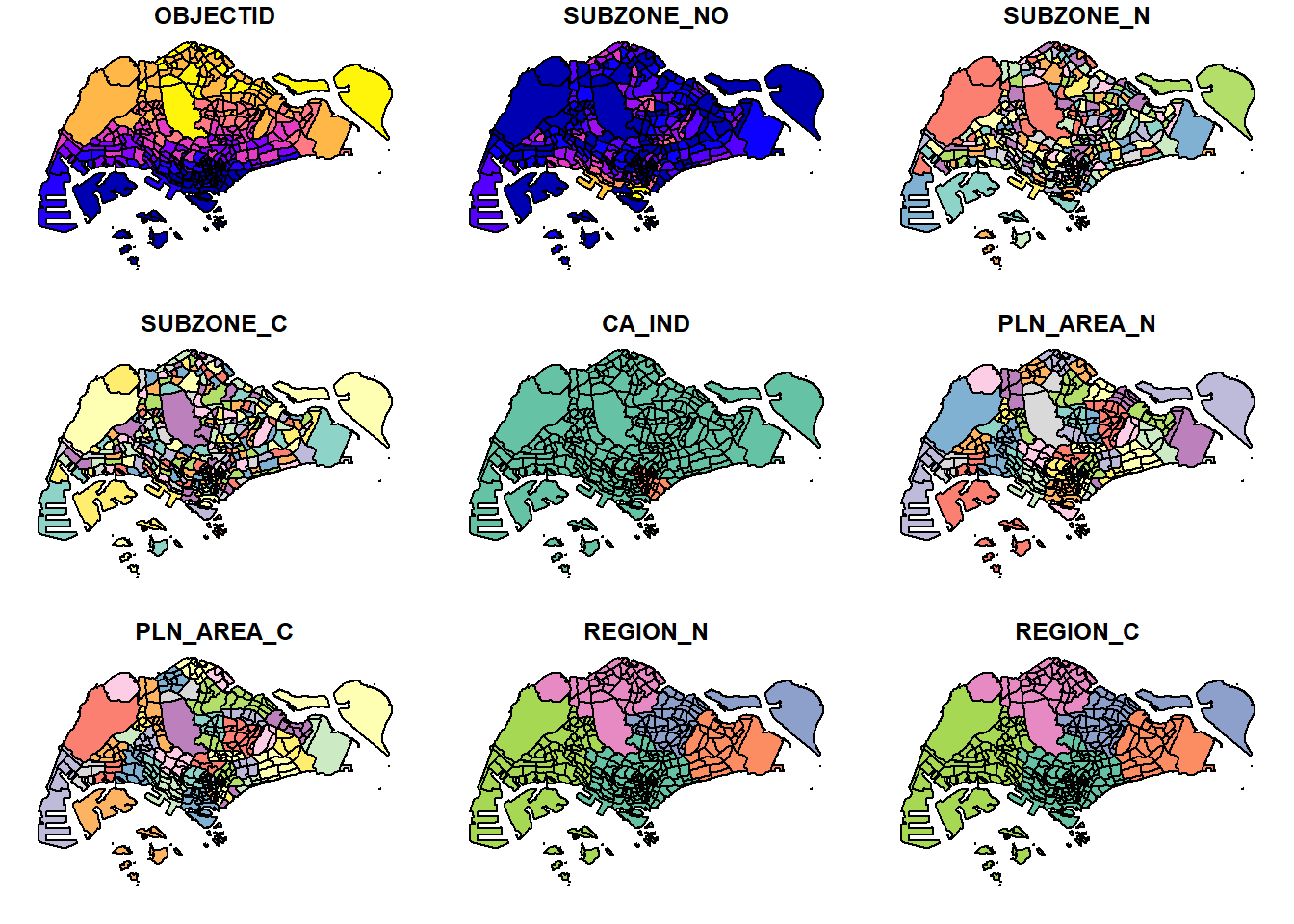
We could also plot only the geometry as shown below.
plot(st_geometry(mpsz))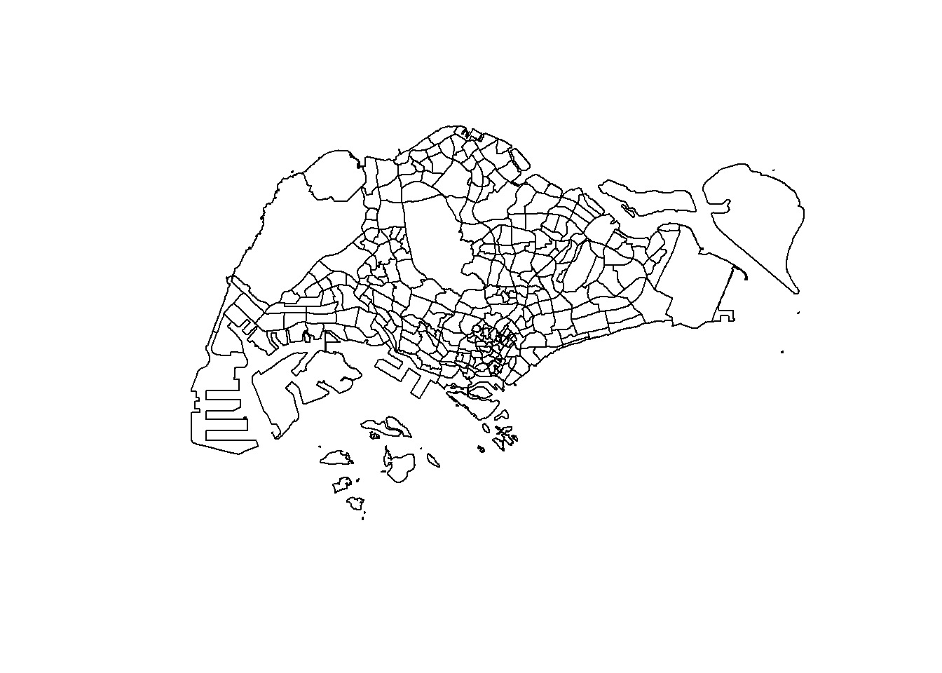
As well as choosing only a specific attribute to be plotted as shown below.
plot(mpsz["PLN_AREA_N"])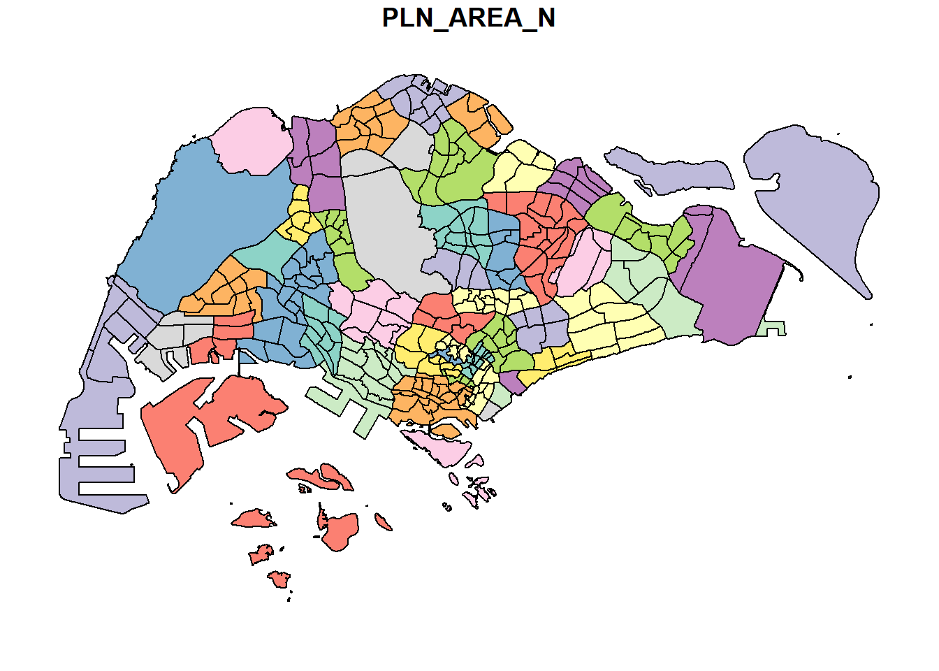
Using plot() for plotting geospatial objects offers a quick look. For high cartographic quality plot, other R package such as tmap should be used.
6 Working with Projection
To perform geoprocessing using two geospatial data, we need to ensure that both geospatial data are projected using similar coordinate system. Projection transformation allows a simple feature data frame to be projected from one coordinate system to another coordinate system.
6.1 Assigning EPSG code to a simple feature data frame
st_crs(mpsz)Coordinate Reference System:
User input: SVY21
wkt:
PROJCRS["SVY21",
BASEGEOGCRS["SVY21[WGS84]",
DATUM["World Geodetic System 1984",
ELLIPSOID["WGS 84",6378137,298.257223563,
LENGTHUNIT["metre",1]],
ID["EPSG",6326]],
PRIMEM["Greenwich",0,
ANGLEUNIT["Degree",0.0174532925199433]]],
CONVERSION["unnamed",
METHOD["Transverse Mercator",
ID["EPSG",9807]],
PARAMETER["Latitude of natural origin",1.36666666666667,
ANGLEUNIT["Degree",0.0174532925199433],
ID["EPSG",8801]],
PARAMETER["Longitude of natural origin",103.833333333333,
ANGLEUNIT["Degree",0.0174532925199433],
ID["EPSG",8802]],
PARAMETER["Scale factor at natural origin",1,
SCALEUNIT["unity",1],
ID["EPSG",8805]],
PARAMETER["False easting",28001.642,
LENGTHUNIT["metre",1],
ID["EPSG",8806]],
PARAMETER["False northing",38744.572,
LENGTHUNIT["metre",1],
ID["EPSG",8807]]],
CS[Cartesian,2],
AXIS["(E)",east,
ORDER[1],
LENGTHUNIT["metre",1,
ID["EPSG",9001]]],
AXIS["(N)",north,
ORDER[2],
LENGTHUNIT["metre",1,
ID["EPSG",9001]]]]mpsz3414 <- st_set_crs(mpsz, 3414)Warning: st_crs<- : replacing crs does not reproject data; use st_transform for
thatst_crs(mpsz3414)Coordinate Reference System:
User input: EPSG:3414
wkt:
PROJCRS["SVY21 / Singapore TM",
BASEGEOGCRS["SVY21",
DATUM["SVY21",
ELLIPSOID["WGS 84",6378137,298.257223563,
LENGTHUNIT["metre",1]]],
PRIMEM["Greenwich",0,
ANGLEUNIT["degree",0.0174532925199433]],
ID["EPSG",4757]],
CONVERSION["Singapore Transverse Mercator",
METHOD["Transverse Mercator",
ID["EPSG",9807]],
PARAMETER["Latitude of natural origin",1.36666666666667,
ANGLEUNIT["degree",0.0174532925199433],
ID["EPSG",8801]],
PARAMETER["Longitude of natural origin",103.833333333333,
ANGLEUNIT["degree",0.0174532925199433],
ID["EPSG",8802]],
PARAMETER["Scale factor at natural origin",1,
SCALEUNIT["unity",1],
ID["EPSG",8805]],
PARAMETER["False easting",28001.642,
LENGTHUNIT["metre",1],
ID["EPSG",8806]],
PARAMETER["False northing",38744.572,
LENGTHUNIT["metre",1],
ID["EPSG",8807]]],
CS[Cartesian,2],
AXIS["northing (N)",north,
ORDER[1],
LENGTHUNIT["metre",1]],
AXIS["easting (E)",east,
ORDER[2],
LENGTHUNIT["metre",1]],
USAGE[
SCOPE["Cadastre, engineering survey, topographic mapping."],
AREA["Singapore - onshore and offshore."],
BBOX[1.13,103.59,1.47,104.07]],
ID["EPSG",3414]]6.2 Transforming the projection of preschool from wgs84 to svy21
Data in geographic coordinate system is not appropriate when distance or/and area measurements are required. In the following, the geographic coordinate system is projected to another coordinate system mathematically.
preschool3414 <- st_transform(preschool, crs = 3414)7 Importing and Converting An Aspatial Data
7.1 Importing the aspatial data
The following listings is an aspatial data which captures the x- and y-coordinates of the data points. Aspatial data is unlike geospatial data which contains information about a specific location on the Earth’s surface.
listings <- read_csv("data/aspatial/listings.csv")Rows: 4252 Columns: 16
── Column specification ────────────────────────────────────────────────────────
Delimiter: ","
chr (5): name, host_name, neighbourhood_group, neighbourhood, room_type
dbl (10): id, host_id, latitude, longitude, price, minimum_nights, number_o...
date (1): last_review
ℹ Use `spec()` to retrieve the full column specification for this data.
ℹ Specify the column types or set `show_col_types = FALSE` to quiet this message.list(listings)[[1]]
# A tibble: 4,252 × 16
id name host_id host_…¹ neigh…² neigh…³ latit…⁴ longi…⁵ room_…⁶ price
<dbl> <chr> <dbl> <chr> <chr> <chr> <dbl> <dbl> <chr> <dbl>
1 50646 Pleasan… 227796 Sujatha Centra… Bukit … 1.33 104. Privat… 80
2 71609 Ensuite… 367042 Belinda East R… Tampin… 1.35 104. Privat… 178
3 71896 B&B Ro… 367042 Belinda East R… Tampin… 1.35 104. Privat… 81
4 71903 Room 2-… 367042 Belinda East R… Tampin… 1.35 104. Privat… 81
5 275343 Conveni… 1439258 Joyce Centra… Bukit … 1.29 104. Privat… 52
6 275344 15 mins… 1439258 Joyce Centra… Bukit … 1.29 104. Privat… 40
7 294281 5 mins … 1521514 Elizab… Centra… Newton 1.31 104. Privat… 72
8 301247 Nice ro… 1552002 Rahul Centra… Geylang 1.32 104. Privat… 41
9 324945 20 Mins… 1439258 Joyce Centra… Bukit … 1.29 104. Privat… 49
10 330089 Accomo@… 1439258 Joyce Centra… Bukit … 1.29 104. Privat… 49
# … with 4,242 more rows, 6 more variables: minimum_nights <dbl>,
# number_of_reviews <dbl>, last_review <date>, reviews_per_month <dbl>,
# calculated_host_listings_count <dbl>, availability_365 <dbl>, and
# abbreviated variable names ¹host_name, ²neighbourhood_group,
# ³neighbourhood, ⁴latitude, ⁵longitude, ⁶room_type7.2 Creating a simple feature data frame from aspatial data frame
In the following, a simple feature data frame is created and the data is transformed into a svy21 projected coordinates system. In the resulting data frame, the longitude and latitude columns will be removed and a new column geometry is added.
listings_sf <- st_as_sf(listings,
                        coords = c("longitude", "latitude"),
                        crs=4326) %>%
st_transform(crs = 3414)glimpse(listings_sf)Rows: 4,252
Columns: 15
$ id <dbl> 50646, 71609, 71896, 71903, 275343, 275…
$ name <chr> "Pleasant Room along Bukit Timah", "Ens…
$ host_id <dbl> 227796, 367042, 367042, 367042, 1439258…
$ host_name <chr> "Sujatha", "Belinda", "Belinda", "Belin…
$ neighbourhood_group <chr> "Central Region", "East Region", "East …
$ neighbourhood <chr> "Bukit Timah", "Tampines", "Tampines", …
$ room_type <chr> "Private room", "Private room", "Privat…
$ price <dbl> 80, 178, 81, 81, 52, 40, 72, 41, 49, 49…
$ minimum_nights <dbl> 90, 90, 90, 90, 14, 14, 90, 8, 14, 14, …
$ number_of_reviews <dbl> 18, 20, 24, 48, 20, 13, 133, 105, 14, 1…
$ last_review <date> 2014-07-08, 2019-12-28, 2014-12-10, 20…
$ reviews_per_month <dbl> 0.22, 0.28, 0.33, 0.67, 0.20, 0.16, 1.2…
$ calculated_host_listings_count <dbl> 1, 4, 4, 4, 50, 50, 7, 1, 50, 50, 50, 4…
$ availability_365 <dbl> 365, 365, 365, 365, 353, 364, 365, 90, …
$ geometry <POINT [m]> POINT (22646.02 35167.9), POINT (…8 Geoprocessing with sf package
In this section, two commonly used geoprocessing functions, namely buffering and point in polygon count will be performed.
8.1 Buffering
The following computes 5-meter buffers (extensions) around cycling paths by using st_buffer() and then computing the corresponding area of the buffers using st_area().
buffer_cycling <- st_buffer(cyclingpath, dist = 5, nQuadSegs = 30)buffer_cycling$AREA <- st_area(buffer_cycling)sum(buffer_cycling$AREA)773143.9 [m^2]8.2 Point-in-polygon count
In the following, we want to identify the number of pre-schools in each planning subzone. This is done by using st_intersects() to identify the pre-schools in each planning subzone and then followed by using length() to calculate the number of pre-schools in each planning subzone.
mpsz3414$`PreSch Count` <- lengths(st_intersects(mpsz3414, preschool3414))We run the following to check the summary statistics of the newly derived PreSch Count field.
summary(mpsz3414$`PreSch Count`) Min. 1st Qu. Median Mean 3rd Qu. Max.
0.000 0.000 2.000 4.207 6.000 37.000 The following lists the planning subzone with the most number of pre-schools.
top_n(mpsz3414, 1, `PreSch Count`)Simple feature collection with 1 feature and 16 fields
Geometry type: MULTIPOLYGON
Dimension: XY
Bounding box: xmin: 23449.05 ymin: 46001.23 xmax: 25594.22 ymax: 47996.47
Projected CRS: SVY21 / Singapore TM
OBJECTID SUBZONE_NO SUBZONE_N SUBZONE_C CA_IND PLN_AREA_N PLN_AREA_C
1 290 3 WOODLANDS EAST WDSZ03 N WOODLANDS WD
REGION_N REGION_C INC_CRC FMEL_UPD_D X_ADDR Y_ADDR
1 NORTH REGION NR C90769E43EE6B0F2 2014-12-05 24506.64 46991.63
SHAPE_Leng SHAPE_Area geometry PreSch Count
1 6603.608 2553464 MULTIPOLYGON (((24786.75 46... 37Next, we want to calculate the density of pre-schools for each planning subzone. We will first derive the area of each planning subzone by using st_area() before computing the density.
mpsz3414$Area <- mpsz3414 %>%
    st_area()
mpsz3414 <- mpsz3414 %>%
mutate(`PreSch Density` = `PreSch Count`/Area * 1000000)9 Exploratory Data Analysis
In this section, we will use ggplot2 functions to create functional and statistical graphs for EDA.
First, we will use a histogram to reveal the distribution of PreSch Density.
hist(mpsz3414$`PreSch Density`)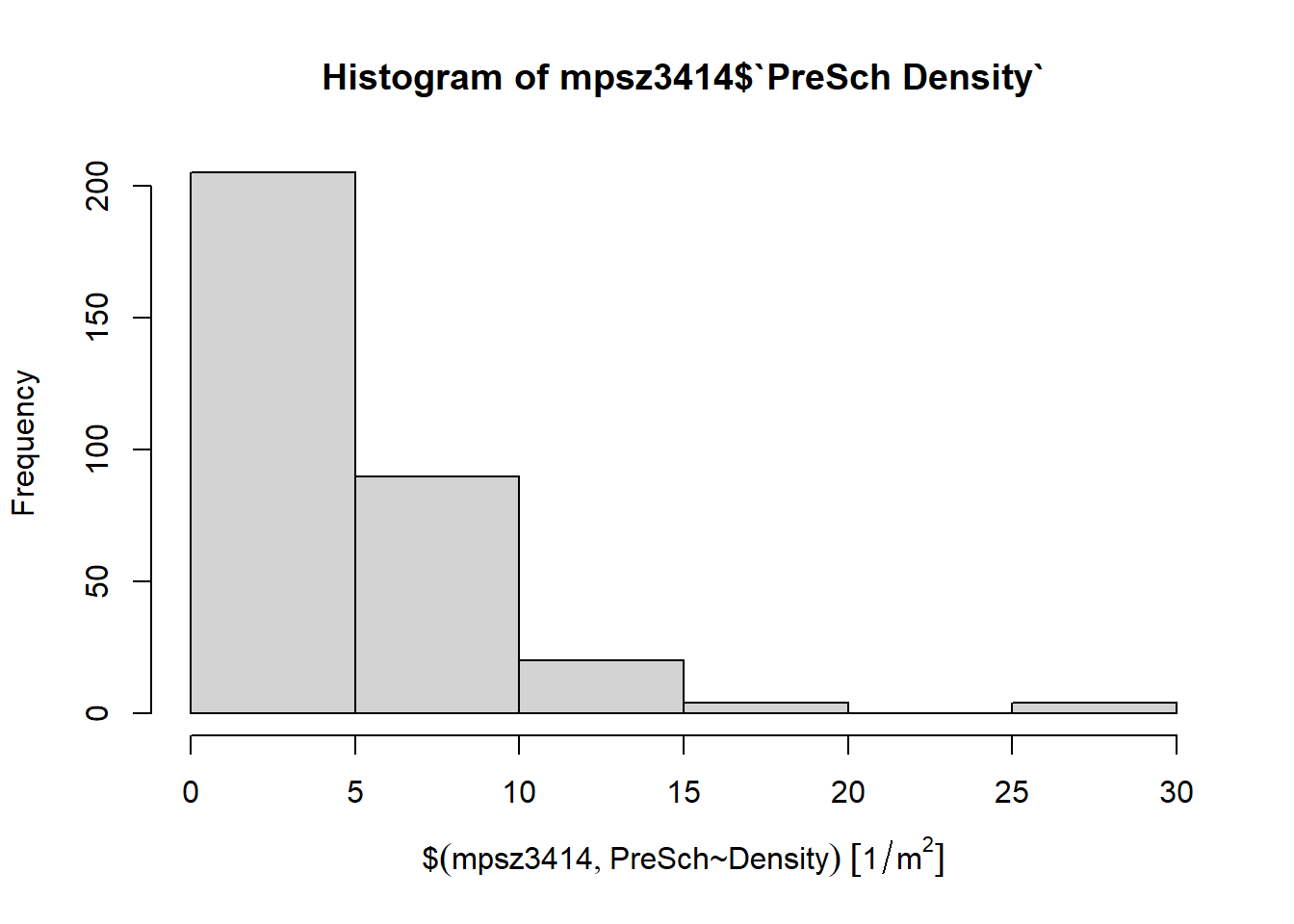
As hist() does not provide much customization, we will use ggplot2 function instead.
ggplot(data = mpsz3414,
       aes(x = as.numeric(`PreSch Density`))) +
    geom_histogram(bins = 20,
                   color = "black",
                   fill = "light blue") +
    labs(title = "Are pre-schools evenly distributed in Singapore?",
         subtitle = "There are many planning subzones with a single pre-school. On the other hand, \nthere are two planning subzones with at least 20 pre-schools.",
         x = "Pre-school density (per km sq)",
         y = "Frequency")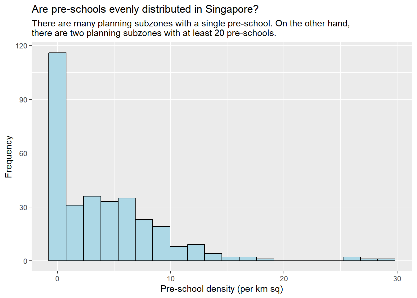
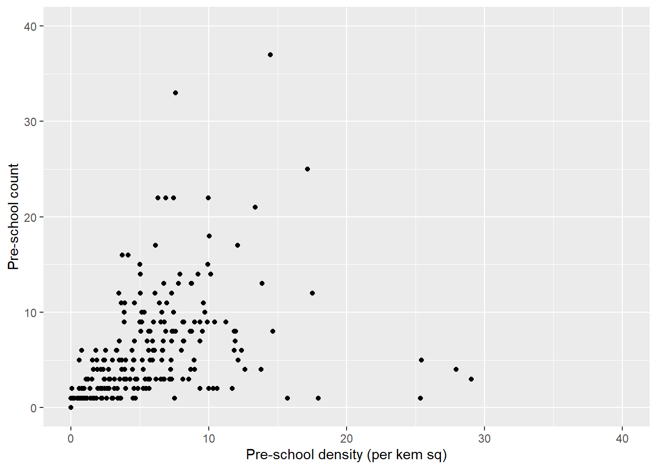
We can also visualize the pre-school count against pre-school density by using a scatterplot.
ggplot(data = mpsz3414,
       aes(x = as.numeric(`PreSch Density`),
           y = as.numeric(`PreSch Count`))) +
    geom_point() +
    labs( x = "Pre-school density (per kem sq)",
          y = "Pre-school count") +
    xlim(0, 40) +
    ylim(0, 40)